Transfer Learning Using Neon

Introduction
In the last few years plenty of deep neural net (DNN) models have been made available for a variety of applications such as classification, image recognition and speech translation. Typically, each of these models are designed for a very specific purpose, but can be extended to novel use cases. For example, one can train a model to recognize numbers and characters in an image and then reuse that model to read signposts in a broader model or a dataset used in autonomous driving.
In this blog post we will:
1. Explain transfer learning and some of its applications
2. Explain how neon can be used for transfer learning
3. Walk through example code that uses neon* for transferring a pre-trained model to a new dataset
4. Discuss the merits of transfer learning with some results
Transfer Learning
Consider the task of visual classification. Convolutional neural networks (CNN) are organized into several layers with each layer learning features at a different scale. The lower level layers recognize low level features such as the fur of a cat or the texture on a brick wall. Higher level layers recognize higher level features such as the body shape of a walking pedestrian or the configuration of windows in a car.
Features learnt at various scales offer excellent feature vectors for various classification tasks. They fundamentally differ from feature vectors that are obtained by kernel-based algorithms developed by human operators because these feature vectors are learnt after extensive training runs. These training runs aim to systematically refine the model parameters so that the typical error between the predicted output, yp=f(xt)(where xt is the observed real world signal and f() is the model), and the ground truth, yt, is made as small as possible.
There are several examples of reusing the features learnt by a well trained CNN. Oquab et. al.
[1] show how the features of an AlexNet model trained on images with a single object can be used to recognize objects in more complex images taken in the real world. Szegedy et. al. [2] show that given a very deep neural network, the features learnt only by half the layers of the network can be used for visual classification. Bell et. al. [3] show that material features (such as wood, glass, etc.) learnt by various pre-trained CNNs such as AlexNet and GoogLeNet can be used for other tangential tasks such as image segmentation. The features learnt by a pre-trained network work so well because they capture the general statistics, the spatial coherence and the hierarchical meta relationships in the data.
Transferring Learning with neon
Neon not only excels in training and inference of DNNs, but also delivers a rich ecosystem with support for requirements surrounding DNNs. For example, you can serialize learned models, load pre- or partially-trained models, choose from several DNNs built by industry experts, and run it in the cloud without any physical infrastructure of your own. You can get a good overview of the neon API here.
You can load pre-trained weights of a model and access them at a per-layer level with two lines of code as follows:
from neon.util.persist import load_obj
pre_trained_model = load_obj(filepath)
pre_trained_layers = pre_trained_model['model']['config']['layers']
You can then transfer the weights from these pre-learnt layer to a compatible layer in your own model with one line of code as follows:
[code]layer_of_new_model.load_weights(pre_trained_layer, load_states=True)[/code]
Then the task of transferring weights from a pre-learnt model to a few select layers of your model is straightforward:
new_layers = [l for l in new_model.layers.layers]
for i, layer in enumerate(new_layers):
if load_pre_trained_weight(i, layer):
layer.load_weights(pre_trained_layers[i], load_states=True)
That’s it! You have selectively transferred your pre-trained model into neon. In the rest of this post, we will discuss: 1) how to structure your new model, 2) how to selectively write code and maximally reuse the neon framework and 3) how to quickly train your new model to very high accuracy in neon without having to go through an extensive new training exercise. We will discuss this in the context of implementing the work of Oquab et. al. [1].
General Scene Classification using Weights Trained on Individual Objects
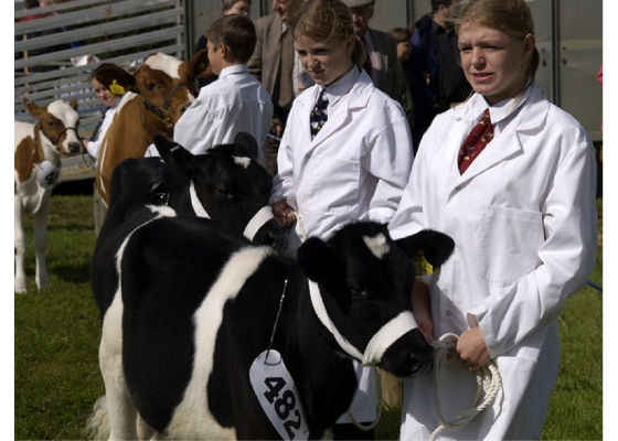
ImageNet is a very popular dataset where the images of the training dataset are mostly representative of individual objects representing 1000 different classes. It is an excellent database for obtaining feature vectors representing individual objects. However, pictures taken in the real world tend to be much more complex with many instances of the objects captured in a single image at various scales. These scenes are further complicated by occlusions. This is illustrated in the below figure where you find many instances of people and cows at varying degrees of scale and occlusion.
Classification in such images is typically done using two techniques: 1) using a sliding multiscale sampler which tries to classify small portions of the image and 2) selectively feeding region proposals discovered by more sophisticated algorithms that are then fed into the DNN for classification. An implementation of the latter approach using Fast R-CNN[4] can be found here. Fast R-CNN also uses transfer learning to accelerate its training speed. In this section we will discuss the former approach which is easier to implement. Our implementation can be found here. Our implementation trains on the Pascal VOC datasetusing an AlexNet model that was pre-trained on the ImageNet dataset.
The core structure of the implementation is simple:
def main():
# Collect the user arguments and hyper parameters
args, hyper_params = get_args_and_hyperparameters()
# setup the CPU or GPU backend
be = gen_backend(**extract_valid_args(args, gen_backend))
# load the training dataset. This will download the dataset
# from the web and cache it locally for subsequent use.
train_set = MultiscaleSampler('trainval', '2007', …)
# create the model by replacing the classification layer
# of AlexNet with new adaptation layers
model, opt = create_model( args, hyper_params)
# Seed the Alexnet conv layers with pre-trained weights
if args.model_file is None and hyper_params.use_pre_trained_weights:
load_imagenet_weights(model, args.data_dir)
train( args, hyper_params, model, opt, train_set)
# Load the test dataset. This will download the dataset
# from the web and cache it locally for subsequent use.
test_set = MultiscaleSampler('test', '2007', …)
test( args, hyper_params, model, test_set)
return
Creating the Model
The structure of our new neural net is the same as the pre-trained AlexNet except we replace its final classification layer with two affine layers and a dropout layer that serve to adapt the neural net trained to the labels of ImageNet to the new set of labels of the Pascal VOC dataset. With the simplicity of neon, that amounts to replacing this line of code (see create_model())
# train for the 1000 labels of ImageNet
Affine(nout=1000, init=Gaussian(scale=0.01),
bias=Constant(-7), activation=Softmax())
with these:
Affine(nout=4096, init=Gaussian(scale=0.005),
bias=Constant(.1), activation=Rectlin()),
Dropout(keep=0.5),
# train for the 21 labels of PascalVOC
Affine(nout=21, init=Gaussian(scale=0.01),
bias=Constant(0), activation=Softmax())
Since we are already using a pre-trained model, we just need to do about 6-8 epochs of training. So we’ll use a small learning rate of 0.0001. Furthermore we will reduce that learning aggressively every few epochs and use a high momentum component because the pre-learned weights are already close to a local minima. These are all done as hyper parameter settings:
if hyper_params.use_pre_trained_weights:
# This will typically train in 5-10 epochs. Use a small learning rate
# and quickly reduce every few epochs.
s = 1e-4
hyper_params.learning_rate_scale = s
hyper_params.learning_rate_sched = Schedule(step_config=[15, 20],
change=[0.5*s, 0.1*s])
hyper_params.momentum = 0.9
else:
# need to actively manage the learning rate if the
# model is not pre-trained
s = 1e-2
hyper_params.learning_rate_scale = 1e-2
hyper_params.learning_rate_sched = Schedule(
step_config=[8, 14, 18, 20],
change=[0.5*s, 0.1*s, 0.05*s, 0.01*s])
hyper_params.momentum = 0.1
These powerful hyper parameters are enforced with one line of code in create_model():
opt = GradientDescentMomentum(hyper_params.learning_rate_scale,
hyper_params.momentum, wdecay=0.0005,
schedule=hyper_params.learning_rate_sched)
Multiscale Sampler
The 2007 Pascal VOC dataset supplies several rectangular regions of interest (ROI) per image with a label for each of the ROI. Neon ships with a loader of the Pascal VOC dataset. We’ll create a dataset loader by creating a class that derives from the PASCALVOCTrain class of that dataset.
We will sample the input images at successively refined scales of [1., 1.3, 1.6, 2., 2.3, 2.6, 3.0, 3.3, 3.6, 4., 4.3, 4.6, 5.] and collect 448 patches. The sampling process at a given scale is simply (see compute_patches_at_scale()):
size = (np.amin(shape)-1) / scale
num_samples = np.ceil( (shape-1) / size)
Since the patches are generated and not derived from the ground truth, we need to assign it a label. A patch is assigned the label of the ROI with which it significantly overlaps. The overlap criteria we choose is that at least 20% of a patch’s area needs to overlap with that of a ROI and at least 60% of that ROI’s area has to be covered by the overlap region. If no ROI or more than one ROI qualifies for this criteria for a given patch we label that patch as a background (see get_label_for_patch()). Typically, the background patches tend to dominate.
During training we bias the sampling to carry more non-background patches (see resample_patches() ). All of the sampling is done dynamically within the __iter__() function of the MultiscaleSampler. This function is called when neon asks the dataset to supply the next mini-batch worth of data. The motivation behind this process is illustrated in figure 4 of [1]
We use this patch sampling method for both training and inference. The MutiscaleSampler feeds neon a minibatch worth of input and label data while neon is not even aware that a meta form of multiscale learning is in progress. Since there are more patches per image than the minibatch size, a single image will feed multiple mini-batches during both training and inference. During training we simply use the CrossEntropyMulti cost function that ships with neon. During inference we leverage neon’s flexibility by defining our own cost function.
Inference
We do a multi-class classification during inference by predicting the presence or absence of a particular object label in the image. We do this on a per-class basis by skewing the class predictions with an exponent and accumulating this skewed value across all the patches inferred on the image. In other words, the score S(i,c) for a class c in image i is the sum of the individual patch scores P(j,c) for that class c, raised to an exponent.
This is implemented by the ImageScores class and the score computation can be expressed with two lines of code (see __call__() ):
exp = self.be.power(y, self.exponent)
self.scores_batch[:] = self.be.add(exp, self.scores_batch)
The intuition behind this scoring technique is illustrated in figures 5 and 6 of [1].
Results
Here are results on the test dataset. The prediction quality is measured with the Average Precision metric. The overall mean average precision (mAP) is 74.67. Those are good numbers for a fairly simple implementation. It took just 15 epochs of training as compared to the pre-trained model that needed more than 90 epochs of training. In addition, if you factor in the hyper-parameter optimization that went into the pre-trained model, we have a significant savings in compute.
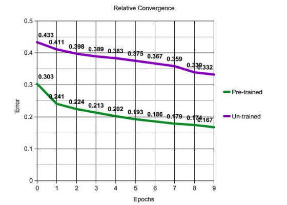
As expected, training converges much faster with a pre-trained model as illustrated in the below graph.
Here are some helpful hints for running the example:
1. Use this command to start a fresh new training run
[code]./transfer_learning.py -e10 -r13 -b gpu –save_path model.prm –serialize 1 –history 20 > train.log 2>&1 &[/code]
2. Use this command to run test. Make sure that the number of epochs specified in this command with the -e option is zero. That ensures that neon will skip the training and jump directly to testing.
[code]./transfer_learning.py -e0 -r13 -b gpu –model_file model.prm > infer.log 2>&1 &[/code]
3. Training each epoch can take 4-6 hours if you are training on the full 5000 images of the training dataset. If you had to terminate your training job for some reason, you can always restart from the last saved epoch with this command.
[code]./transfer_learning.py -e10 -r13 -b gpu –save_path train.prm –serialize 1 –history 20 –model_file train.prm > train.log 2>&1 &[/code]
The pre-trained model that we used can be found here.
A fully trained model obtained after transfer learning can be found here.
You can use the trained model to do classification on the Pascal VOC dataset using AlexNet.
For more such intel IoT resources and tools from Intel, please visit the Intel® Developer Zone
Source:https://software.intel.com/en-us/articles/transfer-learning-using-neon


